A Lower FFT Noise Floor Can Be the Same Noise in Narrower Bins

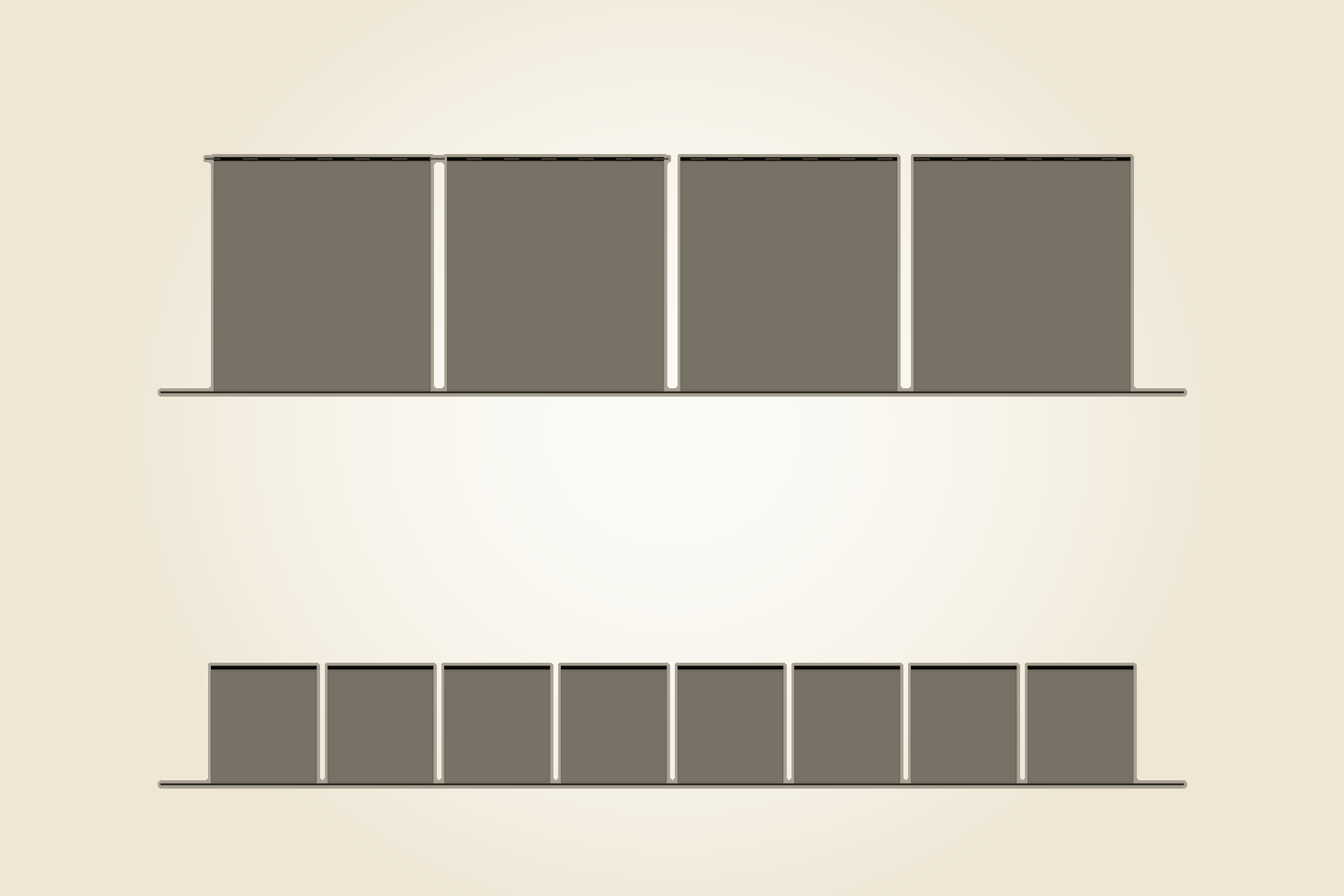
Two FFT plots cover the same frequency range. One shows a noise floor 12 dB lower. It is tempting to call the corresponding DAC, amplifier or interface quieter.

The screenshots alone do not support that conclusion. First establish what each vertical value represents: noise in one FFT bin, noise density normalised to frequency, or noise integrated across a stated bandwidth. These quantities are related, but they are not interchangeable.^[1][2]

Broadband noise is distributed across frequency. Make each FFT bin narrower and each bin contains less of that distributed noise. The trace falls even when the source noise and the total noise across the frequency interval have not changed.^[1]

The comparison that looks obvious

An FFT divides a sampled record into frequency lines. At a sample rate fs and FFT length N, their nominal spacing is:

Δf = fs / N

With sample rate fixed, increasing N reduces bin spacing. For approximately uniform broadband noise, the level in a displayed bin is therefore not a property of the device alone. It also depends on the analyser bandwidth assigned to that bin.^[1][3]

That does not make the lower trace false. It is a real reading under its stated analyser configuration. The mistake is turning it, without further information, into a claim about lower total noise or superior product performance.

Three quantities not to mix

Noise level per bin

This is the level associated with an individual FFT line. For broadband noise, it depends on the bandwidth represented by that line. Narrower bins collect less noise.^[1][2]

Noise spectral density

A density representation expresses noise relative to frequency, commonly per hertz. It can allow comparison across FFT resolutions, but only when the units, window treatment and normalisation are defined correctly. A “dB/Hz” label is useful only if it is genuinely a normalised density.^[4][2]

Integrated RMS noise

Integrated noise sums noise power across a defined frequency range and expresses the result in the relevant level unit. When the question is how much broadband noise lies between two frequency limits, this is generally the useful quantity. The limits, exclusions and processing conditions must still be declared.^[3][2]

Nominal bin spacing is not automatically the effective noise bandwidth. The analysis window changes equivalent noise bandwidth, or ENBW, and can therefore change the correction needed for a rigorous comparison.^[1][5]

An ideal arithmetic example

Consider a stable source of approximately white broadband noise. Keep the sample rate fixed, use the same analysis window and scaling convention, and change only the FFT length from N to 2N.

The nominal bin spacing changes from Δf to Δf/2. In the ideal model, noise power in one bin is approximately:

Pbin ≈ Sn × Δf

Here, Sn is noise power spectral density. Halving Δf halves Pbin. In decibels, the power change is:

10 log10(1/2) ≈ −3.0 dB

So the broadband noise shown in each bin falls by about 3 dB when FFT length doubles. Technical documentation describes this ideal scaling for FFT noise analysis.^[1][2]

Now integrate over the original fixed frequency interval. The longer FFT has twice as many bins in that interval, each carrying half the ideal noise power. Summing their powers returns the same total:

2 × (Pbin/2) = Pbin

A lower displayed floor and unchanged integrated noise are therefore compatible statements. They describe different bandwidths per displayed line, not contradictory physical results.

The example has strict assumptions: approximately uniform broadband noise; a stable source and measurement chain; fixed sample rate; unchanged window and coherent window correction; identical vertical scaling; and integration over the same frequency span. It is a derivation from published relationships, not a measurement made by LineaSonora.^[1][3][2]

Why window and scaling still matter

Real FFT displays are not governed by bin spacing alone. Windows manage spectral leakage, but they also alter the effective bandwidth through which random noise is admitted. Audio Precision, under its stated conventions, lists different window factors, including an ENBW factor of 1.50 for a Hann window and 3.83 for a flat-top window.^[1]

Those values are not universal software constants. Different applications may use different normalisation choices and display amplitude, RMS level, power, a one-sided spectrum or power spectral density. The question is not merely which window was used, but what the program means by its dB value.^[1][4]

FFT averaging is a separate variable. It can make a random floor appear more stable by reducing display variation. Increasing FFT length changes frequency resolution and nominal bin spacing. Both can change a graph’s appearance, but they are not the same operation.^[3]

The important exception: tonal spurs

The approximately 3 dB rule concerns broadband noise distributed over frequency. It should not be applied automatically to mains hum, clock-related spurs, harmonics or test tones.

A discrete component is concentrated rather than uniformly spread across the band. Its apparent height can depend on alignment with FFT bins, spectral leakage, the selected window and the amplitude-correction method. A tone may spread across several lines when it is not coherent with the FFT record, but that is not the same case as broadband noise falling because every bin is narrower.^[3][5]

A tonal spur should therefore be evaluated as a discrete component using an appropriate method. A lower broadband floor does not establish that a spur has fallen, and a changed-looking spur does not automatically indicate a changed circuit.

Checklist before comparing two FFT floors

• Is the sample rate the same? It contributes to bin spacing through Δf = fs/N.^[3]
• Is the FFT length the same? If not, the plots may assign different bandwidths to each bin.^[1]
• Is the window the same, and is ENBW addressed? Nominal bin spacing may not describe effective noise bandwidth.^[1][5]
• What are the vertical units? Determine whether they describe a per-bin level, RMS level, power or density normalised to hertz.^[4][2]
• Are averaging, smoothing, internal filters or automatic scaling involved? These settings can change presentation and interpretation.^[3]
• Is noise integrated over the same stated band? Treat DC, tones and discrete spurs consistently before comparing totals.^[2]
• Does the conclusion stay within the measurement? A graph alone does not establish audibility, which also depends on playback level, spectrum, masking, transducer, environment and a suitable listening protocol.

What the graph can prove

A lower FFT floor can establish that the displayed level is lower under the displayed settings. If those settings include narrower bins, it can be entirely consistent with unchanged integrated broadband noise. The plot does not, by itself, establish that one device has lower physical noise than another.^[1][2]

A defensible comparison either holds sample rate, FFT length, window, scaling and integration bandwidth constant, or converts the results into a properly normalised density or a common integrated-noise result. Without those conditions, the screenshot is incomplete evidence, not a noise ranking.

The useful question is not “Which floor looks lower?” It is: “How much bandwidth does each displayed line represent, and what is the integrated or normalised noise under equivalent conditions?” That is the question the measurement can answer.